I hope that I don’t need to introduce prime numbers to anyone. They are fascinating for all mathematic enthusiasts. We know a lot of prime numbers, but we have no formula to calculate them. Search for the biggest primes is an ongoing competition. People are looking for the biggest primes among the so-called Mersenne Primes. Mersenne Primes are primes that can be expressed as 2ⁿ-1. The record is currently held by 2^82,589,933−1 with 24,862,048 digits, found by GIMPS in December 2018 (more on Wikipedia).

We can find a value of 2^82,589,933-1 online (for example beginning and the end of the number on Wikipedia linked above). But what if we would like to calculate the value ourselves? We have multiple options. For the sake of this article, I selected 2:

bc – an arbitrary precision calculator language

bc is a linux/unix command line calculator that supports arbitrary precision:

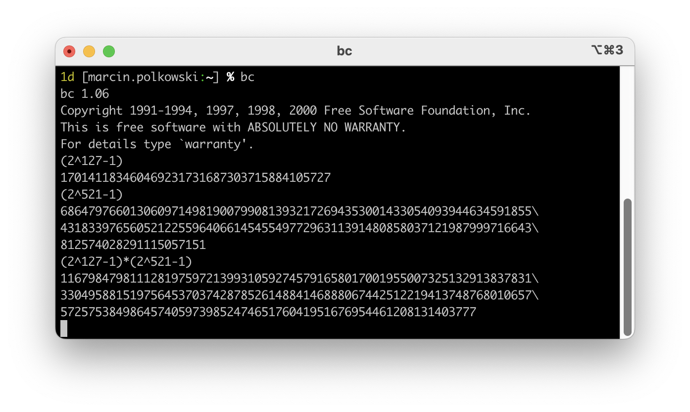
We can run the following in the terminal to calculate the value of 2^82,589,933-1. We use tr and sed to pack the result in one line.

echo "Testing BC:"
time echo "2^82589933-1" \
    | bc \
    | tr "\n" " " \
    | sed 's/\\ //g' \
    > bc.txt

Python

Yes, Python! Python supports arbitrary precision integers by default. There is a slight complication that was added recently for security reasons: we need to increase the default length of the number that can be converted to a string. Let’s consider the following code:

import sys
sys.set_int_max_str_digits(int(3e7))

number = 82589933

print(2**number-1, end=' ')

And run it in the terminal:

echo "Testing Python":
time python python.py > python.txt

It takes python almost 3 hours to compute the result.

Results

Finally, we can confirm that both results are the same:

echo "Comparing Results":
shasum bc.txt
shasum python.txt

Which should give result as following:

Comparing Results:
9abebcdaf11efd28f1797d6b2744cbcb0cc66e52  bc.txt
9abebcdaf11efd28f1797d6b2744cbcb0cc66e52  python.txt

Summary

If you ever need to calculate integers bigger then 64 or 128 bits, now you know how.

Python is great for processing and visualizing data. Today I’d like to share simple tips around plotting data on map using Python.

Let’s consider following example: I want to plot a map of airports around the world. Data for the airports can be obtained from OpenFlights:

        
from io import StringIO
import pandas as pd
import requests

csvString = requests.get("https://raw.githubusercontent.com/jpatokal/openflights/master/data/airports.dat").text
csvStringIO = StringIO(csvString)
airports = pd.read_csv(csvStringIO, sep=",", header=None)
        

This will download the data and create a Pandas DataFrame. We can plot airport locations:

        
import matplotlib.pyplot as plt

ax = plt.subplot(1,1,1)
ax.plot(airports[7], airports[6], 'r.', ms=.5)
plt.axis([-180, 180, -90, 90])
        

Nice plot, but not really a map yet. We need to add some contours. A Global Self-consistent, Hierarchical, High-resolution Geography Database (GSHHG) is a good place to start. You can get data and more info here: http://www.soest.hawaii.edu/pwessel/gshhg/. I recommend downloading “GSHHG coastlines, political borders and rivers in shapefile format (zip archive)”. Now we can plot much nicer map:

        
import geopandas as gp
import matplotlib.pyplot as plt

coastline = gp.read_file('/media/RAID/DATA/GSHHG_2.3.7/GSHHS_shp/f/GSHHS_f_L1.shp')
ax = plt.subplot(1,1,1)

coastline.boundary.plot(ax=ax, edgecolor='black', lw=0.5)

ax.plot(airports[7], airports[6], 'r.', ms=.5)
plt.axis([-180, 180, -60, 85])
        

Or going one step further:

        
import geopandas as gp
import matplotlib.pyplot as plt

coastline = gp.read_file('/media/RAID/DATA/GSHHG_2.3.7/GSHHS_shp/c/GSHHS_c_L1.shp')
borders = gp.read_file('/media/RAID/DATA/GSHHG_2.3.7/WDBII_shp/c/WDBII_border_c_L1.shp')

lakes = gp.read_file('/media/RAID/DATA/GSHHG_2.3.7/GSHHS_shp/c/GSHHS_c_L2.shp')

ax = plt.subplot(1,1,1)

coastline.boundary.plot(ax=ax, edgecolor='black', lw=0.5)
borders.plot(ax=ax, edgecolor='black', lw=0.25)
lakes.boundary.plot(ax=ax, edgecolor='black', lw=0.25)

ax.plot(airports[7], airports[6], 'r.', ms=.5)
plt.axis([-180, 180, -60, 85])
        

Note that in the last example we used “crude resolution” of the coastline and borders – we don’t need much detail for a map in such scale.

Another source of shapefiles with borders that I recommend is GADM. You might be interested in looking at one of my public repositories for more details: GADM-consolidated-shapefile.