Python is great for processing and visualizing data. Today I’d like to share simple tips around plotting data on map using Python.
Let’s consider following example: I want to plot a map of airports around the world. Data for the airports can be obtained from OpenFlights:
from io import StringIO
import pandas as pd
import requests

csvString = requests.get("https://raw.githubusercontent.com/jpatokal/openflights/master/data/airports.dat").text
csvStringIO = StringIO(csvString)
airports = pd.read_csv(csvStringIO, sep=",", header=None)
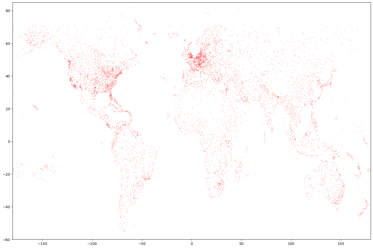
This will download the data and create a Pandas DataFrame. We can plot airport locations:
import matplotlib.pyplot as plt

ax = plt.subplot(1,1,1)
ax.plot(airports[7], airports[6], 'r.', ms=.5)
plt.axis([-180, 180, -90, 90])

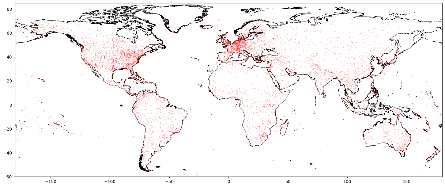
Nice plot, but not really a map yet. We need to add some contours. A Global Self-consistent, Hierarchical, High-resolution Geography Database (GSHHG) is a good place to start. You can get data and more info here: http://www.soest.hawaii.edu/pwessel/gshhg/. I recommend downloading “GSHHG coastlines, political borders and rivers in shapefile format (zip archive)”. Now we can plot much nicer map:
import geopandas as gp
import matplotlib.pyplot as plt

coastline = gp.read_file('/media/RAID/DATA/GSHHG_2.3.7/GSHHS_shp/f/GSHHS_f_L1.shp')
ax = plt.subplot(1,1,1)

coastline.boundary.plot(ax=ax, edgecolor='black', lw=0.5)

ax.plot(airports[7], airports[6], 'r.', ms=.5)
plt.axis([-180, 180, -60, 85])

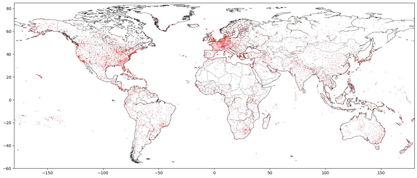
Or going one step further:
import geopandas as gp
import matplotlib.pyplot as plt

coastline = gp.read_file('/media/RAID/DATA/GSHHG_2.3.7/GSHHS_shp/c/GSHHS_c_L1.shp')
borders = gp.read_file('/media/RAID/DATA/GSHHG_2.3.7/WDBII_shp/c/WDBII_border_c_L1.shp')

lakes = gp.read_file('/media/RAID/DATA/GSHHG_2.3.7/GSHHS_shp/c/GSHHS_c_L2.shp')

ax = plt.subplot(1,1,1)

coastline.boundary.plot(ax=ax, edgecolor='black', lw=0.5)
borders.plot(ax=ax, edgecolor='black', lw=0.25)
lakes.boundary.plot(ax=ax, edgecolor='black', lw=0.25)

ax.plot(airports[7], airports[6], 'r.', ms=.5)
plt.axis([-180, 180, -60, 85])

Note that in the last example we used “crude resolution” of the coastline and borders – we don’t need much detail for a map in such scale.
Another source of shapefiles with borders that I recommend is GADM. You might be interested in looking at one of my public repositories for more details: GADM-consolidated-shapefile.


